
VPC Lattice: yet another connectivity option or a game-changer?
12 April 2024 - 4 min. read
Damiano Giorgi
DevOps Engineer


The development of an efficient Machine Learning model is a highly iterative process with continuous feedback loops from previous trials and tests, more akin to a scientific experiment than to a software development project. Data Scientists usually train lots of different models every day trying to get to the most robust model for the scenario they are working on and keeping track of all the tests carried out is often a daunting task even in a single person project.
Amazon offers several tools to help Data Scientists to find the correct set of parameters for their models. Automatic Model Tuning and Amazon SageMaker Autopilot help in exploring quickly and automatically large sections of the phase space, however, these services also contribute to the neverending growth of training jobs parameters and artifacts.
If the project is big enough, multiple engineers are usually involved. Therefore keeping the project as structured as possible, as well as finding ways of sharing all datasets, notebooks, hyperparameters, and results is crucial for success.
The main components of a machine learning project are:
Each team member should always have a clear understanding of which is the latest version of the various components and be able to quickly lookup results and artifacts from previous runs and trials.
To help data scientists with these ML project structuring and management tasks, Amazon released a new service: SageMaker Experiments. This new Amazon Sagemaker component aims to solve this management challenge by giving a unified view for such parameters, training runs, and output artifacts. This new Amazon Sagemaker component aims to solve this management challenge by giving a unified view for such parameters, training runs, and output artifacts.
In this article, we present a real world case where we used SageMaker Experiments extensively.
The project dealt with the clustering of a sparse customer dataset containing several millions of customers in order to understand their behavior. The structure of the dataset and the available features made the clustering algorithm choice, and hyperparameter tuning all but trivial. We tested several types of clustering algorithms (Kmeans, Gaussian mixture, DBSCAN) with different combinations of features. PCA and variable correlation were used to understand the relevant features for clustering.
After several iterations, we found that the most stable result could be found using DBSCAN after dimensionality reduction with UMAP (Uniform Manifold Approximation and Projection). KNN analysis was used to find the optimal radius (eps) for DBSCAN.
UMAP, DBSCAN, and KNN algorithms can be massively accelerated through GPU parallelization.
In order to carry out efficient clustering on our dataset, we decided to use the RapidsAI framework, which includes the CUDA-enabled GPU version of all the algorithms needed for our pipeline. AWS offers several options for GPU enabled Sagemaker ML instances. For our workload we selected an ml.p3.2xlarge for testing and exploration and ml.g4dn.2xlarge for model training.
To install RapidsAI, we can start from the RapidsAI site: Here you can find the installation commands for Conda Python3, which is what will be needed for our testing Sagemaker instance:
conda create -n rapids-0.17 -c rapidsai -c nvidia -c conda-forge \
    -c defaults rapids-blazing=0.17 python=3.7 cudatoolkit=10.1
After that, you’ll need to run the new Jupyter kernel so close and re-open the Notebook, then select “Kernel” -> “Change Kernel”; choose the new RapidsAI kernel you’ve just installed.
Note: Note: every time you stop a Sagemaker instance you lose the custom kernel because it is not part of the standard image shipped with the instance, so you need to install it again with the procedure above.
Typical partitioning methods like K-means or PAM clustering are suitable for finding spherical-shaped clusters or, more in general, convex clusters. They usually work well for compact, well-separated clusters with similar sizes. They are also quite sensitive to the presence of strong anisotropy (noise and outliers) in the data.
Even if good enough for many clustering tasks they are often not the best choice for several real-world situations, in particular they’ll perform terribly bad for:
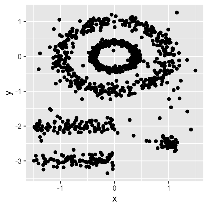
So here comes DBSCAN.
Density-based spatial clustering of applications with noise or in short DBSCAN is a well-known data clustering algorithm that is commonly used in data mining and machine learning.
Based on a dataset of points, DBSCAN groups together those that are close to each other based on distance measurement, typically Euclidean distance, with a threshold based on the minimum number of points. It also marks as outliers those points that are particularly sparse, a.k.a in low-density regions.
DBSCAN algorithm usually requires 2 main parameters:
eps: the local radius for expanding clusters. Think of it as a step size - DBSCAN never takes a step larger than this, and it specifies how close points should be to each other to be considered a part of a cluster.
minPoints: The minimum number of points required to form a dense region (minPts in radius). This is usually strongly related to the minimum cluster size. For example, a value of 100, means that we need at least 100 points to define a cluster if the clusters have well-defined borders and the dataset does not contain random noise.
The parameter estimation is a problem common to every ML task. To choose good values for eps and minPoints some knowledge of the shape of the dataset is usually necessary. Here follow a few general considerations about how to choose reasonable initial eps and minPoints values.
eps: if the eps value chosen is too small, a large part of the data will not be clustered. It will be considered outliers because it doesn't satisfy the number of points to create a dense region. On the other hand, if the value that was chosen is too high, clusters will merge and the majority of objects will be in the same cluster. The eps should be chosen based on the average distance between points of the dataset (we can use a k-distance graph to find it), but in general small eps values are preferable. It should be noted that eps is affected by the dimensionality curse so the more feature you have the bigger will eps be, in fact, the average Euclidean distance in a normalized dataset is proportional to the dimensionality.
minPoints: As a general rule, a minimum minPoints can be derived from a number of dimensions (D) in the data set, as minPoints ≥ D + 1. Larger values are usually better for data sets with noise and will form more significant clusters. The minimum value for the minPoints must be 3, but the larger the data set, the larger the minPoints value that should be chosen.
In order to avoid the dimensionality curse pitfalls and to have more stable and efficient clustering runs a common technique is to use a dimensionality reduction algorithm. In our case, we used correlation analysis for feature selection and then PCA to find which features have more significant impacts on principal components, thus being good candidates as features in the final dataset we’ve used to train our model.
However, directly using PCA for dimensionality reduction led to bad results: the number of principal components required to explain a significant percentage of the dataset variance was quite high and all clustering algorithms performed badly.
The suboptimal PCA performance forced us to look elsewhere for dimensionality reduction. Other commonly used algorithms for dimensionality reduction are t-SNE and UMAP.
Both algorithms perform very slowly in the single-core Scikit-learn implementation on our big dataset, however, things changed dramatically with the RapidsAI GPU CUDA implementation. With the help of the GPU, we were able to carry out dim reduction using the 2 methods in just a few minutes.
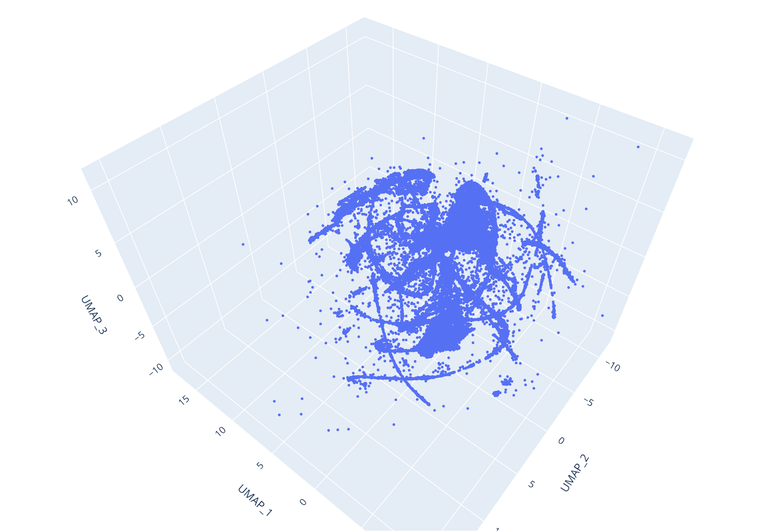
However, UMAP is faster, and, despite while being a novel algorithm, is generally considered to be preferable to t-SNE since it does a good job in preserving both the local and the global structure of the dataset (e.g. see https://towardsdatascience.com/how-exactly-umap-works-13e3040e1668).
Furthermore, UMAP does not use random initialization, so the results are consistent between runs. By reducing the dataset to 3 dimensions, individual clusters could be easily distinguished at glance, and the UMAP trustiness score was very high.
UMAP has a number of important hyper-parameters that influence its performance. These hyper-parameters are:
Measuring how well a ML algorithm is performing is always an essential step in a ML workflow.
While in a supervised machine learning project the way to do so is usually straightforward (train the model on a subset of the data set and test it on another subset), for an unsupervised ML flow, the objective evaluation of the performance is more tricky and even more if the existence and number of clusters are not known nor knowable a priori.
A common way to solve this conundrum is to select one or more performance objective metrics, targets of the clustering output, and check if a given run meets the target performance.
A very general, robust, and widely used metric is the Silhouette score, which is the metric we selected to guide our clustering performance evaluation.
Silhouette score can be used to study the distance between some resulting clusters in a clustering problem; it displays a measure of how close each point in one cluster is to points in the neighboring clusters and thus provides a way to verify parameters like the number of clusters visually.
This measure has a range between -1 and 1.
Silhouette coefficients near 1 indicate that the sample is far away from the neighboring clusters, thus good. A value of 0, instead, says that the point is near to the decision boundary between two near clusters. Finally, negative values indicate that samples might have been assigned to the wrong cluster.
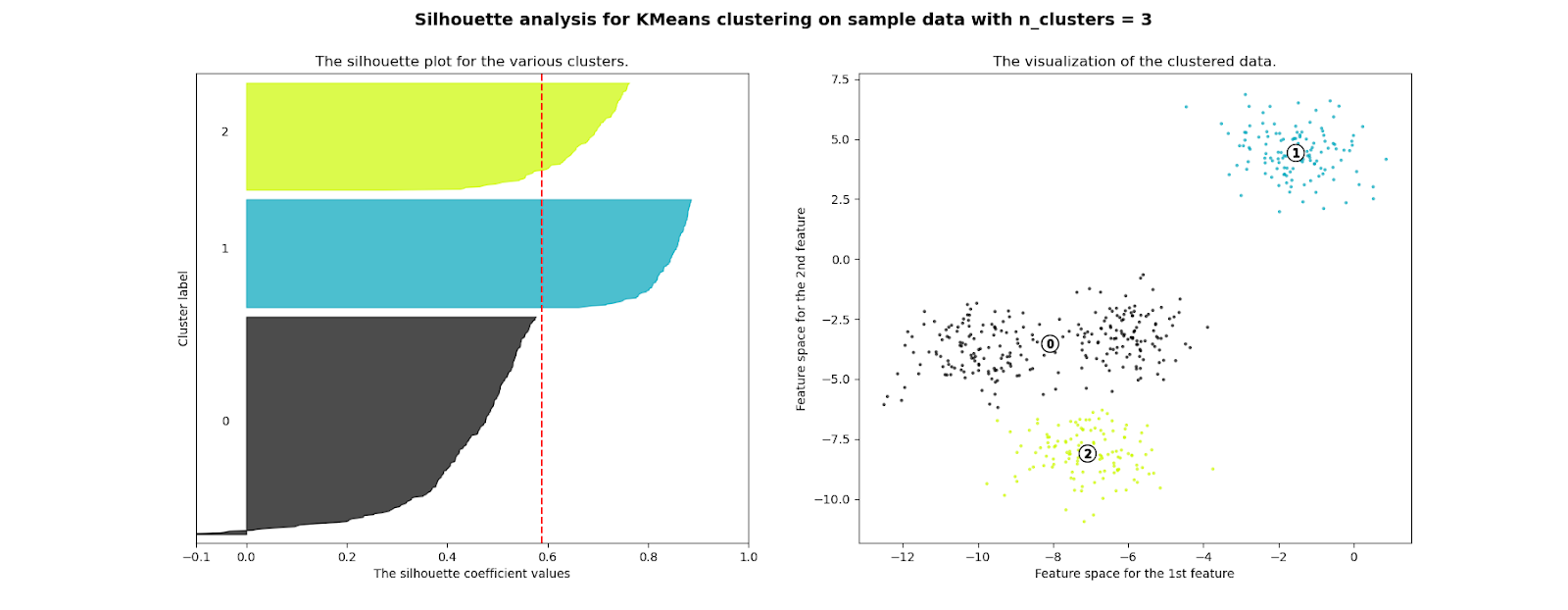
We used this score to verify the quality of our customers’ clusters and to evaluate the performance of different clustering algorithms and sets of hyperparameters.
Completing the clustering workflow took several hundreds of iterations with different data cleaning, heuristics, feature selection, clustering algorithms.
Amazon SageMaker Experiments helps you track iterations to ML models by capturing the input parameters, configurations, and results, and storing them as "experiments". In SageMaker Studio you can browse active experiments, search for previous ones, review them alongside their results, and compare those results.
The goal of SageMaker Experiments - with its Python API - is to make it as simple as possible to create those experiments, populate them with trials, and run analytics across trials and experiments.
You can run complex queries to quickly find the past trial you’re looking for. You can also visualize real-time model leaderboards and metric charts.
In the course of this article, you’ll be guided through SageMaker Experiment’s features and setup by following the real world scenario we faced.
In order for us to use SageMaker Experiments, we first need to get access to Sagemaker Studio, to do so we created some users - one for each collaborator - in AWS Console.
You need to have the right permissions to access SageMaker services through the console, if you have, you just need to click on the left sidebar of the service page and access SageMaker Studio property panel. There you’ll find the “Add user” button to create a new user.
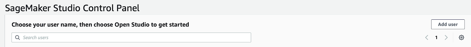
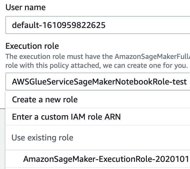
The creation of a user is straightforward: just give a name and a valid IAM role like in the example below and then you’re good to go. See the image below for clarity:
This is a simple yet crucial point: when managing a project, complex like a Machine Learning one, constant checks with the customer are extremely important. Giving him the ability to easily assert the results of every experiment, makes it easier to have feedback and significantly improves the chances of a satisfactory result for the ML project.
Before starting to understand how Experiments works, let’s define some key concepts you must know:
The goal of SageMaker Experiments is - of course - to make it as simple as possible to access and manipulate experiments, populate them with trials, and moreover doing analytics over trials and experiments to make ponderate decisions.
To help with this task, AWS offers a Python SDK - containing logging and analytics APIs - to integrate Experiments in notebooks.
Before starting to describe the process in details, just a clarification: we used the most elastic approach in dealing with Machine Learning problems with SageMaker, which is bring your own container: that means we define our ML code in scripts passed to an Estimator, which runs on custom images pushed to AWS ECR.
Why do this extra work, instead of using precooked material from AWS? Because we needed extra flexibility in dealing with our problem, and in general - you’ll see that - apart from extreme rare cases, you’ll probably end up doing the same thing with your use-case.
Real world scenarios involving companies have very specific conditions that can be addressed with higher precision, only when the algorithms and models are tailored and fine-tuned on that specific problem.
In Jupyter Notebooks, users can add automatisms using SageMaker API; when defining an Estimator for evaluating a model, it is now possible to add an Experiment definition, this way we are basically linking the operation to a tuple in the Experiment console in SageMaker Studio.
In our clustering process this capability was important, because we had the explicit need to give weekly updates, on how our models were performing. Usually this is, as said, a good practice to help create a clear understanding of the problem with the client, and in general, to avoid confusion.
Before passing an experiment to an estimator, as stated by the official AWS documentation, we need to generate it from scratch; in a new Jupyter notebook cell we write these lines:
import sagemaker
from smexperiments.experiment import Experiment
from sagemaker import get_execution_role
from sagemaker.session import Session

experiment_name="my-TestExperiment"

role = get_execution_role()
session=Session()
sm_client=session.boto_session.client('sagemaker')

experiment = None
for exp in  Experiment.list():
    if exp.experiment_name==experiment_name:
        experiment = Experiment.load(experiment_name=experiment_name,sagemaker_boto_client=sm_client)
        print(f"Experiment {experiment_name} is loaded!")
        break;

if experiment == None:
    experiment = Experiment.create(
        experiment_name = experiment_name,
        description = "My Test Experiment",
        tags = [{'Key': 'project', 'Value': 'customer-segmentation'}]
    )
    print(f"Experiment {experiment_name} is created!")
In these lines of code we are describing a new experiment and not only: if the experiment already exists in the experiment list, which depends on the credentials of the user logged on Jupyter, that experiment is loaded, instead of creating a new one.
Why did we do this? Because we wanted to divide experiments by categories, then use trials to group different training jobs. This way you can keep things cleaner.
An experiment can then be added to an Estimator, but before doing so, Trials must be created and added to the experiment itself (that’s why we can also load an existing experiment).
Trials are groups in which every training occurrence is kept. They are defined in an experiment and can be used to divide and keep different training jobs, with different sets of parameters, separated and clean.
We did this because we tried a great number of hyperparameters sets in order to fine tune the models, partly also because we had a very sparse initial dataset which was very difficult to analyze in terms of clustering.
To add a Trial to a SageMaker Experiment, here is an example code to use in a cell below the one with the Experiment initialization.
from smexperiments.trial import Trial
from smexperiments.trial_component import TrialComponent
from smexperiments.tracker import Tracker

import time
from time import strftime

trial_create_date = strftime("%Y-%m-%d-%H-%M-%S")
trial_name ="test-trial-{}".format(trial_create_date)

trial = None
try:
    trial = Trial.load(trial_name, sagemaker_boto_client=sm_client)
    print(f"Trial {trial_name} is loaded!")
except:
    trial = Trial.create(trial_name = trial_name,
                         experiment_name = experiment.experiment_name,
                         tags = [{'Key': 'my-experiments', 'Value': 'trial 1'}])
    print(f"Trial {trial_name} is created!")
In this case - to be able to distinguish among all the trials - we generate the trial name dynamically, which is a common pattern; you can make it depending on the category of the trial or on the parameters involved. Just be aware of the trial name characters limit (120 characters), so don’t make it too long and avoid special characters as they are not permitted.
Now that we have added a Trial to an experiment it is possible to add it to an estimator to make it available from the SageMaker Studio IDE.
Estimators handle end-to-end Amazon SageMaker training and deployment tasks. It’s a Python class that defines all the characteristics of a training. To add Experiment support just add an extra line of code to an estimator’s definition like in the example below:
estimator.fit(
inputs={"train":sagemaker.session.s3_input(s3_data=data_location)},
       wait=True,
       logs='All',
       experiment_config={
             "ExperimentName":experiment.experiment_name,
             "TrialName" : trial.trial_name,
             "TrialComponentDisplayName" : "Training",
       }
)
Basically, when we run the .fit() method to start a training job, SageMaker recognizes the experiment_config parameter and links that particular job to the Sagemaker Studio Experiment dashboard.
This demonstrates how simple it is to create an experiment, but you also need to define a Tracker, in order to actually push information to the Experiment Dashboard.
To effectively push information to the SageMaker Studio Dashboard you need to setup a Tracker. A tracker is basically a logger which takes different inputs and sends them to specific tabs of the Experiment console, depending on the method used.
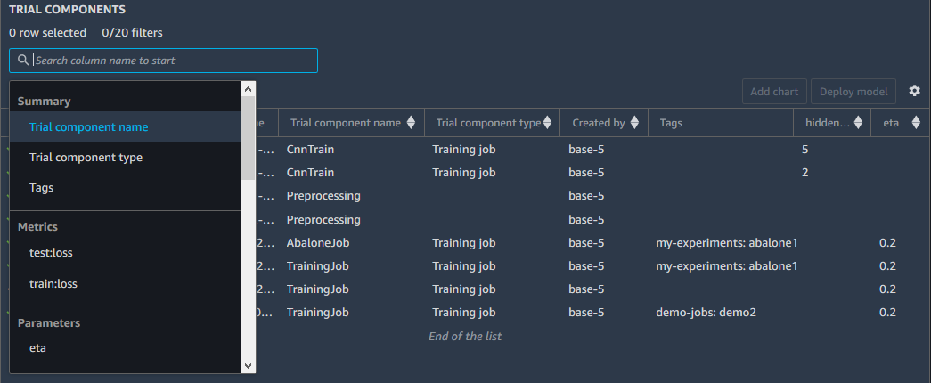
Thanks to the tracker and some predefined logs offered by SageMaker Experiments, you can end up with a comprehensive description of your trial like in the image below:
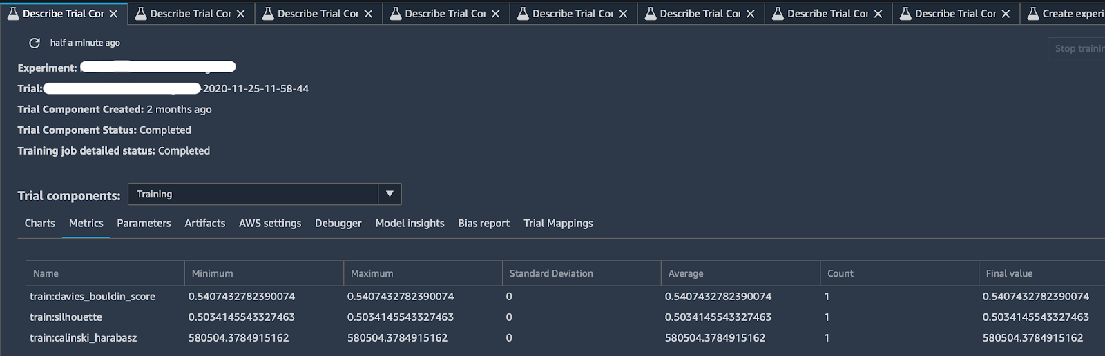
Clicking on the “Describe Trial Component” tab, you can choose any column headings to see information about each trial component, in particular:
A Tracker can - and typically must - be added to the estimator script which contains your Machine Learning logic. After defining the entry point parameters (i.e. the args for your script), you can load a Tracker this way:
# Loading Sagemaker Experiments Training Tracker
tracker=tracker.Tracker.load()
After this line of code it is now possible to start sending information towards SageMaker Studio. In our case we used 3 specific tracker methods:
tracker.log_parameters({ "param1": NUM, "param2": NUM, ...})
Which is used to send the extra parameters to the “Parameters” tab in the dashboard of that particular trial.
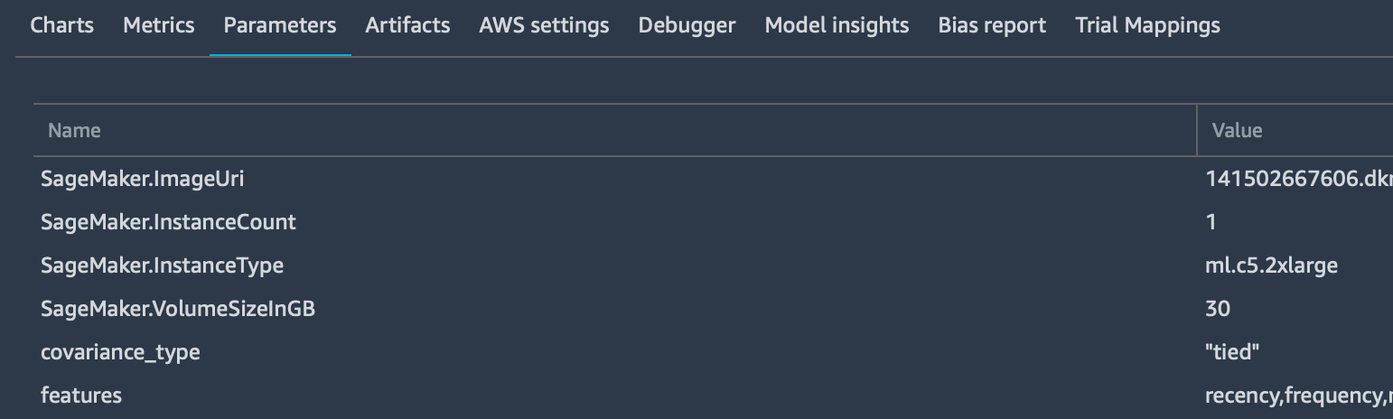
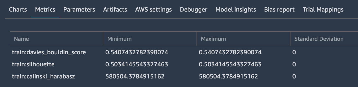
tracker.log_input(“key”, “value”, media_type=TYPE)
Which is used to log as many input parameters as you want, also specifying the media type to allow previewing them - if possible - in the browser. These parameters will be added to the “Metrics” tab:
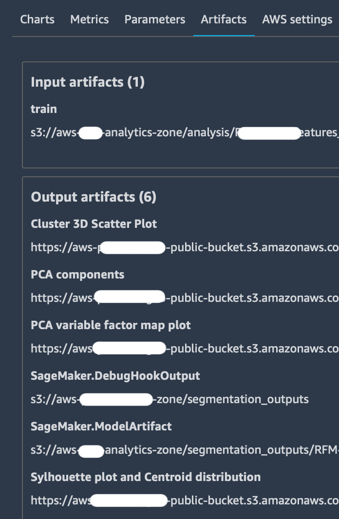
tracker.log_output(name="Some link name", media_type="s3/uri", value=s3_uri)Is used to send specific outputs to the “Artifacts” tab which already contains Amazon S3 bucket storage locations for the input dataset and the output model.
Finally, always remember to close a tracker before ending the script.
tracker.close()
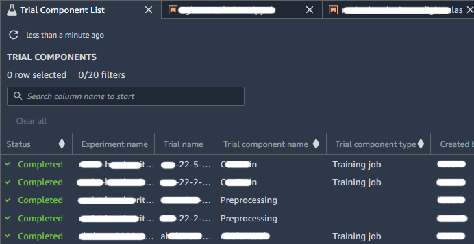
As stated also by AWS documentation, you can compare experiments, trials, and trial components by opening them in the Studio Leaderboard. In this screen you can do the following actions:
When you have one or more experiments you can open the Leaderboard to compare the results. Choose the experiments or trials that you want to compare; right-click on one of the elements, and then click on “Open in trial component list”. The Leaderboard will open and you’ll be presented with a list of associated Experiments entities as shown in the image below:
From our experimentation we found that the Tracker can only be used when the Estimator is launched in online mode, i.e. specifying an instance type which is not “local”. It means that you’re running the training on a newly created instance, instead of running it directly on the instance where the notebook resides.
In this article, we have seen how we leveraged the new capabilities offered by Amazon SageMaker Experiments to smother the clustering of a remarkable amount of data. In our journey, we used these new features to better share results in our team and with the client, and to coordinate the effort of the engineers involved.
We didn’t go too much in depth with the characteristics of SageMaker Experiments, but we shared the most important traits as we would like to encourage the reader in trying and playing by himself.
Along the way, we’ve also seen how to use two interesting clustering algorithms: DBSCAN and UMAP. These are better suited for finding groups of similar data when the original dataset is sparse and inhomogeneous, but require a CUDA enabled instance.
Finally, we have also briefly discussed the key concept of “bring your own container” in SageMaker, which we found, fundamental to complete our analysis: as we have said, when dealing with complex real life scenarios, pre-cooked algorithms offered by AWS SageMaker are not flexible enough.
To conclude we hope you enjoyed the reading, for any questions feel free to contact us, to talk about Machine Learning or any other topic related to the amazing world of Cloud Computing!
Stay tuned for more articles about Machine Learning! See you in 14 days on #Proud2beCloud!